Chemical Engineering Simulation

Roger G.E. Franks

Jon Paul Van Buskirk

PC-based process simulation has been increasingly popular in the last four decades. Advances in hardware and software applications driven by the demand of personal computing has had a positive influence on existing technologies. The need for both steady-state and dynamic simulators in the chemical industry becomes greater as environmental, quality and safety issues grow with the expanding industries. Companies are beginning to recognize the benefits that simulators can provide including research and development, plant design and retrofitting, and plant operations. Combined with modeling, control and optimization, simulation can enable companies to make better engineering and business decisions in both plant design and operations.

As processes become more complex, incorporating varying degrees of automation, there is an increasing need in design and operations using simulators for process understanding. Modern analysis usually involves mathematical modeling either on a bench or pilot scale prior to a commercial plant. Two broad classifications include steady state and dynamic models. The attention to detail requires a solution based on the accuracy of the basic data obtained from scaled-down studies; therefore, steady state and dynamic simulators are highly effective when actual process data is used in physical property prediction, mass and energy balances, kinetics, transportation, etc. Process simulation leads to a deeper understanding of the internal mechanisms and characteristics of the process.

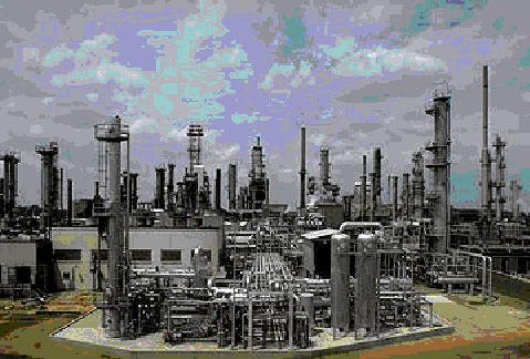
Picture 1: Chemical Plant showing the diversity of equipment types.

The Chemical Industry is diverse and requires several desktop tools for process understanding and improvement. Figure 1 shows the vast array of piping and equipment in a chemical process. Equipment can be modeled on an individual basis or using groups of common functionality. The number of model types and complexity is also diverse and modeling methods can range from a first principle approach to data intensive methods such as genetic algorithms or artificial neural nets. Data systems can range into the tens of thousands of variables and modeling methods based on actual data is ultimately required to adequately represent these systems. A model representation is required for operations, control and optimization of the process. Benefits include enhanced quality, safety, environmental, and economic controls.

The term simulation, when used in chemical engineering, has been extended to almost every area that requires the use of a computer to calculate large sets of simultaneous equations. The system models most frequently encountered are as follows.

(a) Steady-state flows, composition, temperatures and pressures are calculated for complex continuous chemical processes. These flowsheet calculations provide the key data that are used to size process equipment, an essential step in the design of a chemical plant.

(b) The dynamic behavior of variables is usually modeled in a multiloop recycle process or in a transient batch operation. These dynamic simulations involve the solution of large sets of simultaneous algebraic and differential equations, are used to solve problems in process control and batch process yield optimization.

(c) An important area of system simulation, which has had a major impact in the process industry, is the use of computers as sophisticated on-line controllers that provide extensive monitoring of process variables, and is also used as feedback supervisory controls.

(d) Another application area is the use of computers in design engineering, where the designer is able to duplicate a three-dimensional drawing of an existing or projected design of a chemical plant. The piping layout, vessel location, foundations, and so on can be easily changed, while the effects of these changes verified and working drawings printed out at the plant site.

(e) Many other specialized system simulation programs are frequently used by design specialists to solve problems in the control of rotating machinery such as centrifugal compressors and steam turbines or electric motors. Also, steady-state pressures and flows in large piping networks need to be calculated in order to size process and service piping. Simulations of complete compressor and piping systems for a wide range of operations, including, but not limited to, start-up, normal operation at steady and varying load conditions, including anti-surge, normal and emergency shutdowns, and safety valve relieving conditions are used for evaluation of compressor design and performance.

1. Steady-State Simulation

Some of the larger industrial chemical companies have been using internally developed proprietary computer programs to construct flowsheets of steady-state processes. One program, DESIGN II (formerly ChemShare), was made generally available and has been used in numerous industrial locations for more than 30 years. This program performs steady-state material and energy balances, estimates equipment costs and carries out economic evaluations for variety of pipeline and processing applications. The simplified windows approach to the creation of process models integral to DESIGN II allows engineers to use complicated and rigorous process design-base calculations from a proven benchmark. It contains almost all physical property components and 38 world crude properties already stored in libraries. DESIGN II for Windows may be applied to synthetic-fuel processes and conventional liquid-vapor streams, typical in oil refining and chemical plant operations. It is also applicable to processes involving the flow of unconventional materials requiring unusual process equipment. Since other simulation programs can be either difficult to use, very expensive or both, DESIGN II has become a corporate standard for many industries across the world.

Most simulation programs use the well-accepted calculation method termed sequential modular. The programs consists of a library of subroutines, each containing the equations describing the function of a particular type of process equipment such as a condenser, heat exchanger or pump. The information flow connecting these units consists of a large stream array, each stream containing the stream compositions, flow rates, temperatures and other properties. The user selects the modules representing the process, assigns stream numbers and specifies physical property data for the chemical components in the system. The program proceeds to solve each unit sequentially, and for recycle loops or counter-current processes, it repeats this calculation to achieve an overall balance using an appropriate convergence technique. Any special conditions can be introduced into the program by including a custom coding prepared by the user who also has the choice of selecting the most appropriate equation-of-state calculation to be used. The advantage of using these structured programs is that they allow a user with minimal skills in computer programming or numerical technology to operate a high complex, sophisticated program and obtain flowsheet values for large process systems. The following is a typical scenario for the use of a steady-state simulation:

Case Study 1 - Facilities design using a Steady-State Simulator:

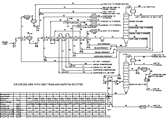
Figure 1: Steady-state simulation for process design and performance of a refinery.

A fundamental approach is required for new facilities design since data is not available. In the process industries, a simulator is used for mass, momentum, and energy balances and for chemical or physical property generation. The fluid components are selected, and the equipment and streams laid out in a flow sheet fashion. From this information, the simulator solves for the process conditions in a sequential method. The results provide the information necessary for equipment sizing, costing, predictive maintenance and optimization. Figures 1 and 2 are representations of process flow diagrams using the steady-state simulator from Design II for Windows™. Figure 1 depicts a simulator for rigorous process design of a refinery. Figure 2 is an example of a debutanizer column design. Objectives of simulations include design and optimize process operations to maximize energy savings while reducing production costs and risk.

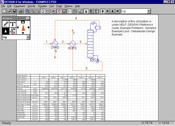
Figure 2: Debutanizer example for column design and optimization.

2. Dynamic Simulation

Chemical processes generally operate on an unsteady basis. Ideally, they are maintained at their desired operating levels by the use of closed-loop feedback controllers, which provide satisfactory operation most of the time. Problems arise when abnormal conditions occur or when the process is subjected to sudden disturbances or unexpected equipment failures. In a highly coupled and interactive process such disturbances, if not properly stabilized by the control system, can sometimes result in a catastrophic shutdown of the process, or damage to equipment, with consequent loss of production until the process can be restarted.

Simulation of the process and its control systems, either in the design phase or during operation, has proved a valuable method of uncovering potential weaknesses in control configuration when the process is subjected to disturbances. The same simulation can then be used to devise improved control schemes or operating strategies, and sometimes to suggest modifications to equipment that will ensure that the process is sufficiently stable when subjected to disturbances. Owing to the size and complexity of the chemical plant, these simulations must be conducted on personal computers. The simulation model consists of a large number of algebraic and differential equations, grouped in sets, each set representing the dynamic performance of each unit operation in the process being simulated. Such a model is similar to a steady-state model, but takes account of mass and energy accumulation in various vessels which give rise to the differential equations that describe how process variables such as compositions, flows and temperature in a vessel change with time when the operating conditions in the vessel change.

Assembling complex computer simulations of chemical processes is greatly facilitated by the use of a library of prepackaged computer program modules, integrated with an operating system, each module representing the dynamic behavior of most of the more common unit operations. Program libraries are available with DYFLO (Franks 1972), one of the most widely used, and in addition to unit operation modules they also contain mathematical routines that allow the programmer to construct special programs for unique process modules not included in the library. The latest versions of these programs incorporate automatic internal procedures for handling the differential equation "stiffness" that invariably occurs in such systems: for example DYFLO2 (Franks 1982). The following is a scenario for the use of a Dynamic simulator:

Case Study 2 - Facilities Design using a Dynamic Simulator:

Dynamic transitions in a chemical process cannot be accurately modeled using a steady-state simulator. For all practical purposes, a dynamic simulator integrated with a full physics package based on a time dependent method should be used for transitional data analysis. As with the steady-state simulator dynamics must include all physical/chemical property calculations with a flow sheet generator interface. Figure 3 is an example of a reactor system utilizing the QMC DYFLO Program for reactor kinetics. The model is in a dynamic time domain and can also be used for tanks, pumps, compressors / expanders, heat exchangers, pipes & valves, control valves, controllers, reactors / combustors, distillation, etc. The technology has been successfully used in chemical processes for over 30 years with many benefits for system analysis and robust methods for actual operational evaluation of both steady-state and transitional, or dynamic conditions.

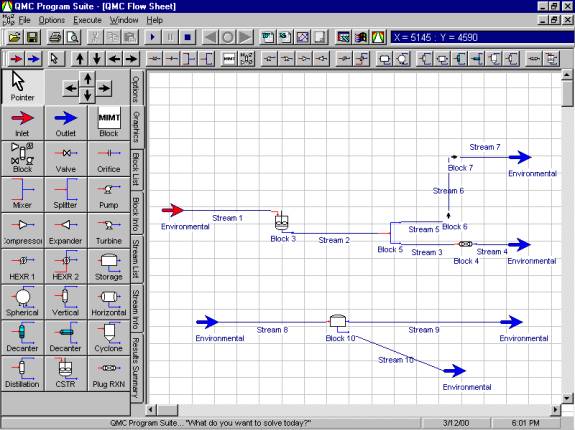
Figure 3: Flow sheet(s) for a reactor system utilizing the QMC DYFLO for reactor kinetics

Case Study 3 - Facilities Design using Detailed Sizing Programs:

From steady-state and/or dynamic simulation, a detailed design of equipment can be reviewed and verified. In the Chemical Industry, this equipment includes piping, control valves, safety valves, flow meters, pumps, compressors, heat exchangers, decanters, gas-liquid separation vessels, etc. Figure 4 provides the results of a control valve sizing procedure. Depicted is the control valve flow coefficient, termed CV, versus flow rate. Also shown is the limit of flows for this control valve system. Figure 5 is a detailed design program to size a Counterflow Shell and Tube heat exchanger. Detailed equipment design typically gives thorough results, i.e. mechanical design, stress analysis, etc., for final design generating spec sheets for the vendor.

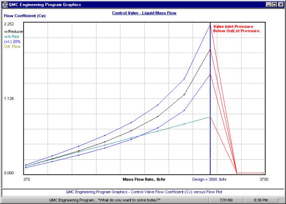
Figure 4: Rating plot for sizing results of a control valve sizing procedure (CV versus flow rate).

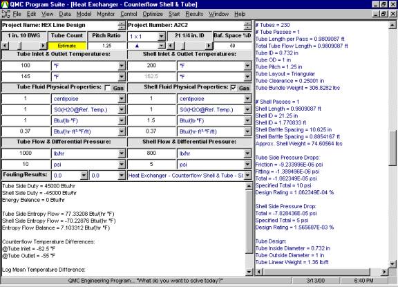
Figure 5: Detailed design programs are used to size equipment for mechanical and physical performance analysis.

Case Study 4 - Modified Iterative Measurement Test Method:

An enhancement to simulation in order to determine the measured data accuracy is the Modified Iterative Measurement Test Method (Serth and Heenan, AIChE Journal, Vol. 32, 1986). The QMC MIMT Program solves the linear and non-liner data-reconciliation/gross-error-detection problem. For a given set of measured data, the program generates a reconciled data set, i.e., one, which is consistent with all applicable constraints, such as material balance or model based requirements. It also generates a list of measurements, which are suspected of being grossly in error, as well as estimates of the correct values of the suspect measurements. Typical applications include total material balances, temperatures, pressures, etc. for chemical processes or plants, steam-metering systems in plants and refineries, and natural gas distribution systems. However, the program is applicable to any data set for which the measured variables are related to one another by a system of linear or non-linear algebraic equations. Complex networks of pipes, tanks and process components are shown in Figure 6.

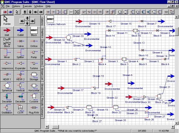
Figure 6: Complex networks of pipes and process equipment using MIMT to verify critical measurements.

Case Study 5 - Economic Optimization:

Economic reporting provides a procedure to monitor and optimize production costs. The steps are: a) Perform economic balance, b) Model economics using plant data, and c) Minimize production costs using a model optimizer. Economic optimization and reporting can run in on-line and off-line modes.

The economic balance can be done using spreadsheet functions or a transform calculation program. The transform calculations should use both fixed and variable costs for a more complete economic evaluation.

This procedure is shown in Figure 7. Provided in this figure are the Plant data, calculated economic variables, and associated economic equations. Results are saved to a spreadsheet for future analysis.

For this example a small part of the total process, a reactor system, is used for economic analysis. This approach allows focus to different operating areas and allows for localized optimization of individual unit operations. A global approach will help select which areas of the plant will provide the major profit improvement. The global approach will also provide a monitoring check on realized production cost savings.

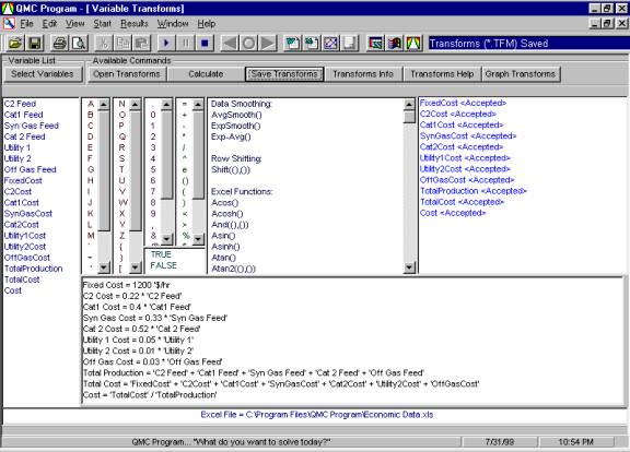
Figure 7: Economic Evaluation using Plant Data Set.

The (sorted) cost per hour is given in Figure 8. As shown on this graph, a wide range of operating costs exists. This is due to a wide range in production rates and the effects of fixed and utility costs. For this process, it is best to maximize production rates to minimize product costs.

A model of the cost can include applicable process data such as pressures, temperatures, flows, and concentrations. The model can then be adjusted to minimize the cost with respect to these variables when used as system set points. The results of this modeling procedure are also shown in Figure 8 (where Ya are the actual values and Yp are the model-predicted values for cost per pound of production.)

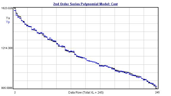
Figure 8: Results for modeling process production costs.

With this model, many methods are available for optimization. This provides the set points that minimize costs. This can be done for both on-line and off-line applications. In this case, the optimum occurs at maximum production rates. However, this maximum production may be limited by several factors, such as hardware, raw materials availability, or off-site limitations. Therefore, a constrained optimization algorithm should also be applied.

Other modeling methods to be considered include genetic algorithms, neural net, evolutionary, etc., or simulation methods adapted towards the respective industry. The modeling technique selected should come with an optimizer that can handle a wide range of applications. The maximum benefits of modeling are when an optimization procedure can be utilized.

Synopsis:

This article reviewed several case studies involving design, simulation, data reconciliation and optimization of both steady-state and dynamic chemical processes. These technologies provide a basis leading to process understanding and improvement. These case studies are in reference to actual field applications and include steady-state simulation, dynamic simulation, detailed equipment design and performance, Modified Iterative Measurement Test method and economic evaluation and optimization.

It was also shown how simulation, modeling and optimization methods work together in a unified approach to design and improve process. When these methods are used for monitoring, control, and optimization, a quality, safety, environmental, and economic advantage can be maintained along with peak operating levels.

The applications of these techniques are not limited to the process industries. They can be adapted to any industry utilizing data systems. Implementation will provide a definite technology advantage, and promote a logical and systematic approach for continuous process improvement to meet desired goals.

For a demonstration copy of any programs listed in this article, please contact QMC at 281.359.4471 or QMC@QMC.net.

_________________________________________

Jon Paul Van Buskirk, MSChE, is a Principal with Quality Monitoring & Control. He has experience in refineries, petrochemical and polymer industries and may be reached at QMC@QMC.net.

Roger G.E. Franks, M.Sc., is an Associate of Quality Monitoring & Control. Formerly with DuPont, he pioneered the technology of modeling and computer simulation of chemical process dynamics for 35 years. He authored the basic text in this field and created the DYFLO program, used for simulating chemical process units, now in general use worldwide.

Bibliography

Franks R G E 1972 Modeling and Simulation in Chemical Engineering, Wiley, New York

Franks R G E 1982 DYFLO update: DYFLO2. In: Summer Computer Simulation Conf. Society for Computer Simulation La Jolla, California, pp. 507-13

Thambynayagam R K M, Wood R K. Winter P 1981 DPS-AN Engineers' s tool for dynamic process analysis Chem. Eng. (London) 365, 58-65

Serth, R W, Heenan, W A, Gross Error Detection and Data Reconciliation in Steam-Metering Systems, AIChE Journal, Vol. 32, No. 5, 733-742